design_proposed

esis.flights.f2.optics.design_proposed(grid=None, axis_channel='channel', num_distribution=11)

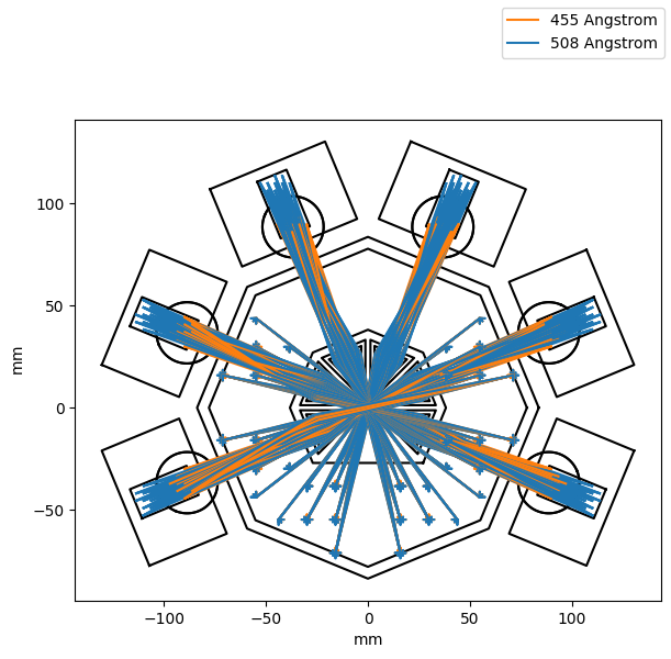
Load the proposed optical design for ESIS 2.

Parameters:

• grid (None | ObjectVectorArray) – sampling of wavelength, field, and pupil positions that will be used to characterize the optical system.

• axis_channel (str) – The name of the logical axis corresponding to changing camera channel.

• num_distribution (int) – number of Monte Carlo samples to draw when computing uncertainties

Return type:

Instrument

Examples

Plot the rays traveling through the optical system, as viewed from the front.

import numpy as np
import matplotlib.pyplot as plt
import astropy.units as u
import astropy.visualization
import named_arrays as na
import optika
import esis

grid = optika.vectors.ObjectVectorArray(
    wavelength=na.linspace(-1, 1, axis="wavelength", num=2, centers=True),
    field=0.99 * na.Cartesian2dVectorLinearSpace(
        start=-1,
        stop=1,
        axis=na.Cartesian2dVectorArray("field_x", "field_y"),
        num=5,
    ),
    pupil=na.Cartesian2dVectorLinearSpace(
        start=-1,
        stop=1,
        axis=na.Cartesian2dVectorArray("pupil_x", "pupil_y"),
        num=5,
    ),
)

instrument = esis.flights.f2.optics.design_proposed(
    grid=grid,
    num_distribution=0,
)

with astropy.visualization.quantity_support():
    fig, ax = plt.subplots(
        figsize=(6, 6.5),
        constrained_layout=True
    )
    ax.set_aspect("equal")
    instrument.system.plot(
        components=("x", "y"),
        color="black",
        kwargs_rays=dict(
            color=na.ScalarArray(
                ndarray=np.array(["tab:orange", "tab:blue"]),
                axes="wavelength",
            ),
            label=instrument.system.grid_input.wavelength.astype(int),
        ),
    );
    handles, labels = ax.get_legend_handles_labels()
    labels = dict(zip(labels, handles))
    fig.legend(labels.values(), labels.keys());

References to esis.flights.f2.optics.design_proposed
design_proposed