Throughput#

This report investigates the efficiency of each ESIS optical component and estimates the total sensitivity of the optics (not including the sensor).

To accomplish this, we trace a grid of rays through the system and compute the ratios of the intensity of the unvignetted rays. This allows us to compute the average efficiency over the whole FOV, instead of just the on-axis efficiency.

[1]:

import matplotlib.pyplot as plt
import astropy.visualization
import named_arrays as na
import esis

Load the optical design

[2]:

instrument = esis.flights.f1.optics.design_single(num_distribution=0)
instrument.wavelength = na.linspace(-1, 1, axis="wavelength", num=101)

Trace rays through the optical design

[3]:

rays = instrument.system.raytrace().outputs

WARNING: function 'sqrt' is not known to astropy's Quantity. Will run it anyway, hoping it will treat ndarray subclasses correctly. Please raise an issue at https://github.com/astropy/astropy/issues. [astropy.units.quantity]
/opt/hostedtoolcache/Python/3.11.13/x64/lib/python3.11/site-packages/astropy/units/quantity.py:653: RuntimeWarning: divide by zero encountered in divide
  result = super().__array_ufunc__(function, method, *arrays, **kwargs)

Create a list with the names of each surface

[4]:

surface_names = [s.name for s in instrument.system.surfaces_all]

Isolate the name of the logical axis indicating different surfaces

[5]:

axis_surface = instrument.system.axis_surface

Compute the index of each surface

[6]:

index_source = 0
index_primary = surface_names.index(instrument.primary_mirror.surface.name)
index_grating = surface_names.index(instrument.grating.surface.name)
index_filter = surface_names.index(instrument.filter.surface.name)

Compute the intensity of the rays at each surface

[7]:

axis_sum = instrument.field.axes + instrument.pupil.axes
kwargs_sum = dict(
    axis=axis_sum,
    where=rays.unvignetted[{axis_surface: ~0}],
)
intensity_source = rays.intensity[{axis_surface: index_source}].sum(**kwargs_sum)
intensity_primary = rays.intensity[{axis_surface: index_primary}].sum(**kwargs_sum)
intensity_grating = rays.intensity[{axis_surface: index_grating}].sum(**kwargs_sum)
intensity_filter = rays.intensity[{axis_surface: index_filter}].sum(**kwargs_sum)

Compute the efficiency of each surface by taking intensity ratios

[8]:

efficiency_primary = intensity_primary / intensity_source
efficiency_grating = intensity_grating / intensity_primary
efficiency_filter = intensity_filter / intensity_grating
efficiency_total = intensity_filter / intensity_source

/opt/hostedtoolcache/Python/3.11.13/x64/lib/python3.11/site-packages/astropy/units/quantity.py:653: RuntimeWarning: invalid value encountered in divide
  result = super().__array_ufunc__(function, method, *arrays, **kwargs)

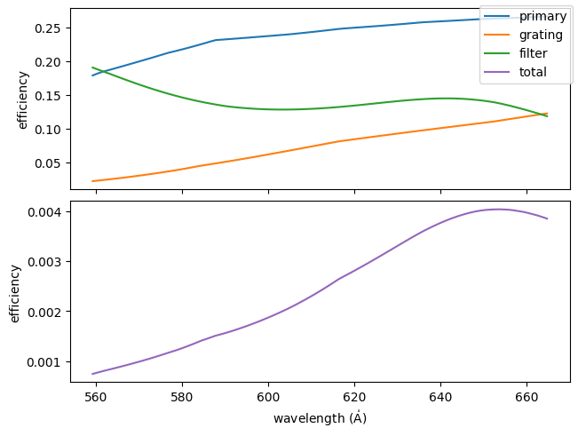
Plot the efficiencies as a function of wavelength.

[9]:

with astropy.visualization.quantity_support():
    fig, ax = plt.subplots(
        nrows=2,
        sharex=True,
        constrained_layout=True,
    )
    na.plt.plot(
        instrument.wavelength_physical,
        efficiency_primary,
        ax=ax[0],
        label=instrument.primary_mirror.surface.name,
        color="tab:blue",
    )
    na.plt.plot(
        instrument.wavelength_physical,
        efficiency_grating,
        ax=ax[0],
        label=instrument.grating.surface.name,
        color="tab:orange",
    )
    na.plt.plot(
        instrument.wavelength_physical,
        efficiency_filter,
        ax=ax[0],
        label=instrument.filter.surface.name,
        color="tab:green",
    )
    na.plt.plot(
        instrument.wavelength_physical,
        efficiency_total,
        ax=ax[1],
        label="total",
        color="tab:purple",
    )
    fig.legend()
    ax[1].set_xlabel(f"wavelength ({ax[1].get_xlabel()})")
    ax[0].set_ylabel("efficiency")
    ax[1].set_ylabel("efficiency")

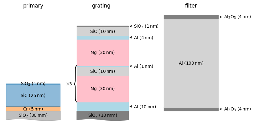
Plot a schematic of the three multilayer stacks to compare

[10]:

with astropy.visualization.quantity_support():
    fig, ax = plt.subplots(
        ncols=3,
        sharey=True,
        figsize=(8,4),
        constrained_layout=True,
    )
    instrument.primary_mirror.material.plot_layers(ax=ax[0])
    instrument.grating.material.plot_layers(ax=ax[1])
    instrument.filter.material.plot_layers(ax=ax[2])
    ax[0].set_title(instrument.primary_mirror.surface.name)
    ax[1].set_title(instrument.grating.surface.name)
    ax[2].set_title(instrument.filter.surface.name)
    ax[0].set_axis_off()
    ax[1].set_axis_off()
    ax[2].set_axis_off()
    ax[2].autoscale()

Throughput#

This Page