design_visible

esis.flights.f2.optics.design_visible(grid=None, axis_channel='channel', num_distribution=11)

Load a visible-light version of the ESIS-II design.

This is a model of the visible-light alignment gratings. Since the flight rulings are too fine to be tested with visible light, each science grating is paired with a visible-light alignment grating whose ruling spacing is scaled so that a HeNe laser reproduces the flight geometry.

This model starts with design() and multiplies every coefficient of the grating ruling spacing polynomial by the ratio

\[\frac{d_\text{vis}(y)}{d(y)} = \frac{\lambda_\text{HeNe}}{\lambda_c},\]

where \(\lambda_\text{HeNe} = 632.8\) nm is the wavelength of a HeNe laser and \(\lambda_c\) is the center of the EUV passband. From the grating equation, preserving \(\lambda / d(y)\) at every point on the face of the grating means that a HeNe laser diffracted into first order by the alignment grating follows the same path through the instrument as \(\lambda_c\) diffracted by the science grating.

Parameters:

• grid (None | ObjectVectorArray) – sampling of wavelength, field, and pupil positions that will be used to characterize the optical system.

• axis_channel (str) – The name of the logical axis corresponding to changing camera channel.

• num_distribution (int) – number of Monte Carlo samples to draw when computing uncertainties

Return type:

Instrument

Examples

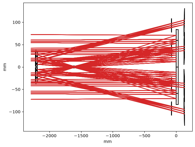
Plot the rays traveling through the visible-light optical system, as viewed from the side.

import matplotlib.pyplot as plt
import astropy.visualization
import named_arrays as na
import esis

# Load the visible-light instrument into memory
instrument = esis.flights.f2.optics.design_visible(num_distribution=0)

# Lower the number of field and pupil samples
# for clearer plotting
instrument.field.num = 3
instrument.pupil.num = 3

with astropy.visualization.quantity_support():
    fig, ax = plt.subplots(constrained_layout=True)
    instrument.system.plot(
        components=("z", "x"),
        color="black",
        kwargs_rays=dict(
            color="tab:red",
        ),
    );

References to esis.flights.f2.optics.design_visible
design_visible
Grating Specifications / Visible Alignment Gratings