Image Simulation

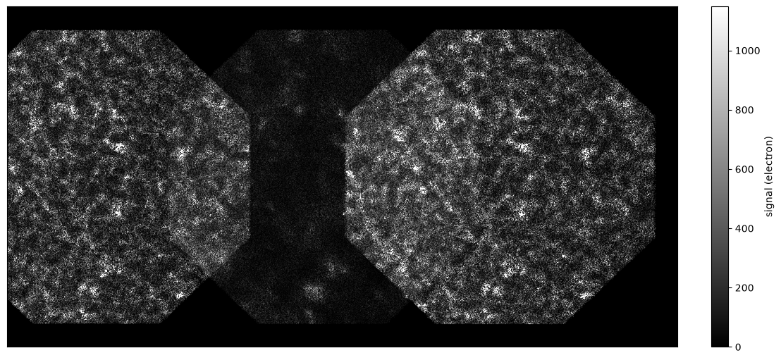
The Atmospheric Imaging Assembly (AIA) [Lemen et al., 2012] on the Solar Dynamics Observatory [Pesnell et al., 2012] is a NASA satellite that continuously observes the Sun in extreme ultraviolet (EUV). Since some of the EUV channels that AIA observes are close in temperature to the lines that ESIS observes, we can use AIA observations to simulate ESIS images. In this notebook, we select the AIA images from during the ESIS-I 2019 flight and simulate sythetic images using the ideal ESIS design.

import warnings
import matplotlib.pyplot as plt
import named_arrays as na
import esis

warnings.filterwarnings("ignore")

Define the logical axis corresponding to changes in time.

axis_time = "time"

Define the logical axis corresponding to changes in line-of-sight velocity.

axis_velocity = "velocity"

Define the logical axes corresponding to changes in position on the disk of the Sun.

axis_x = "detector_x"
axis_y = "detector_y"

Load the sythetic scene composed of AIA images. Here, we use the scene_aia() function, which recreates the brightest three lines in the ESIS passband.

scene = esis.flights.f1.data.synth.scene_aia(
    axis_time=axis_time,
    axis_detector_x=axis_x,
    axis_detector_y=axis_y,
    axis_velocity=axis_velocity,
    limit=1,
)

Load a single channel of the ideal ESIS optical model.

instrument = esis.flights.f1.optics.design_single(num_distribution=0)

Reduce the number of rays traced per field angle so that this tutorial has a reasonable runtime. This number should be increased to simulate research-quality images.

instrument.pupil.num = 2

Also halve the number of pixels in each axis to increase the signal-to-noise ratio of the final image.

sensor = instrument.camera.sensor
sensor.width_pixel = 2 * sensor.width_pixel
sensor.num_pixel_x = sensor.num_pixel_x // 2
sensor.num_pixel_y = sensor.num_pixel_y // 2

Image the sythetic scene using our model of the ESIS optical system.

%%time
images = instrument.system.image(
    scene=scene[{axis_time: 0}],
    axis_wavelength=axis_velocity,
    axis_field=(axis_x, axis_y),
)

CPU times: user 1min 19s, sys: 23.1 s, total: 1min 42s
Wall time: 1min 29s

Display the simulated image.

fig, ax = plt.subplots(
    figsize=(11, 5),
    constrained_layout=True,
)
vmax = images.outputs.percentile(99.9).value
img = na.plt.pcolormesh(
    images.inputs.position.x,
    images.inputs.position.y,
    C=images.outputs.sum(("wavelength", axis_velocity)).value,
    cmap="gray",
    vmin=0,
    vmax=vmax,
)
ax.set_xticks([])
ax.set_yticks([])
ax.set_aspect("equal")
plt.colorbar(img.ndarray.item(), label=f"signal ({images.outputs.unit})");