Design & Specifications

This report inspects the ESIS-II optical design and evaluates its performance.

The ESIS-II optical design has been modified from the ESIS-I design to have higher resolution and different target wavelengths. The changes from ESIS-I are as follows:

• The target wavelengths have changed to Ne VII 46.5 nm and Si XII 49.9 nm.

• The primary mirror is moved back by 6 holes on the optical bench.

• The gratings are moved forward by 2 holes on the optical bench.

• The filter position and orientation has been adjusted to account for the shallower beam.

To account for these changes, the angle, radius of curvature, and the ruling parameters of the grating need to be adjusted. This design used differential_evolution() to compute these parameters.

import numpy as np
import matplotlib.pyplot as plt
import astropy.units as u
import astropy.visualization
import named_arrays as na
import optika
import esis

Start by loading a single channel of the optical design to investigate its performance.

instrument = esis.flights.f2.optics.design_single(num_distribution=0)

Lower the number of field angles from the default to make the results easier to interpret.

instrument.field.num = 5

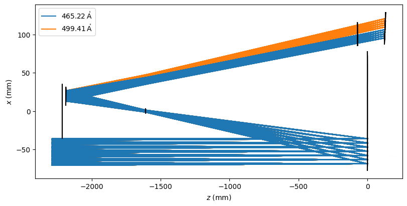
Plot the rays associated with this single channel.

with astropy.visualization.quantity_support():
    fig, ax = plt.subplots(
        figsize=(8, 4),
        constrained_layout=True,
    )
    instrument.system.plot(
        ax=ax,
        components=("z", "x"),
        color="black",
        kwargs_rays=dict(
            color=na.ScalarArray(
                ndarray=np.array(["tab:blue", "tab:orange"]),
                axes="wavelength",
            ),
            label=instrument.wavelength.to_string_array(),
            zorder=-instrument.wavelength.value,
        ),
    )
    ax.set_xlabel(f"$z$ ({ax.get_xlabel()})")
    ax.set_ylabel(f"$x$ ({ax.get_ylabel()})")

    handles, labels = ax.get_legend_handles_labels()
    by_label = dict(zip(labels, handles))
    ax.legend(by_label.values(), by_label.keys())

WARNING: function 'sqrt' is not known to astropy's Quantity. Will run it anyway, hoping it will treat ndarray subclasses correctly. Please raise an issue at https://github.com/astropy/astropy/issues. [astropy.units.quantity]

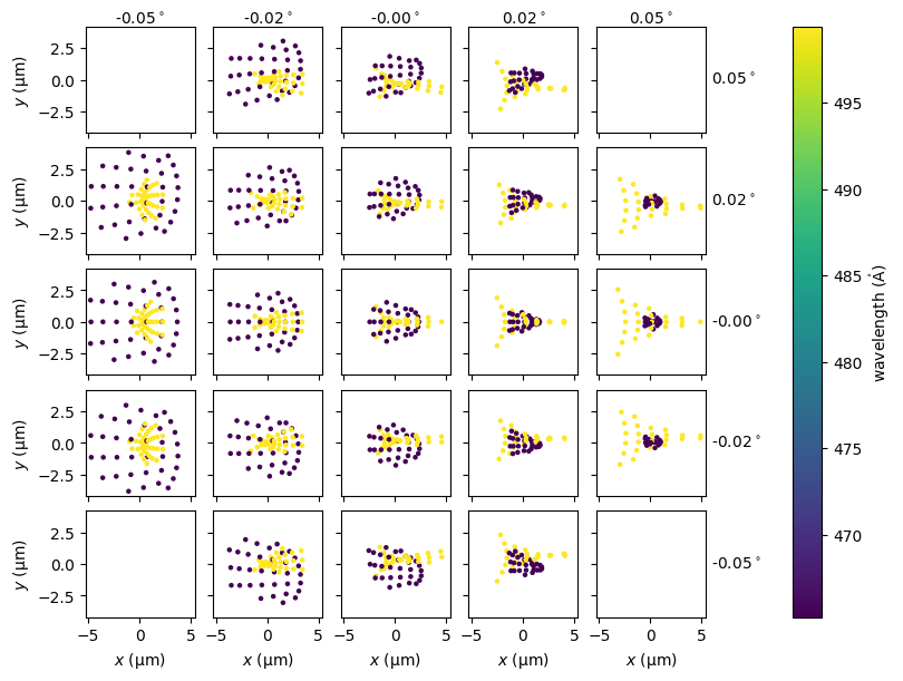
Spot Diagram

Plot the spot diagram associated with this channel to inspect the PSF of the system.

instrument.system.spot_diagram();

Primary Footprint Diagram

Now, we would like to plot a diagram showing the footprint of the beam on the primary mirror. To do this, we will define a dense array of field points that goes almost to the edge of the FOV,

field = na.Cartesian2dVectorLinearSpace(
    start=-0.99,
    stop=+0.99,
    axis=na.Cartesian2dVectorArray("fx", "fy"),
    num=11,
)

and a denser array of pupil points that also goes almost to the edge.

pupil=na.Cartesian2dVectorLinearSpace(
    start=-0.99,
    stop=+0.99,
    axis=na.Cartesian2dVectorArray("px", "py"),
    num=41,
)

Now, load the model of the full ESIS-II instrument, including all channels, with a much denser grid of rays.

instrument_full = esis.flights.f2.optics.design(
    grid=optika.vectors.ObjectVectorArray(
        wavelength=instrument.wavelength,
        field=field,
        pupil=pupil,
    ),
    num_distribution=0,
)

We will also rotate the instrument 22.5 degrees counter clockwise so that the borders of the primary are parallel to the vertical and horizontal.

instrument_full.roll = 22.5 * u.deg

Finally, we will rotate the primary mirror 180 degrees about the \(y\) axis so that we view it from the front.

transformation = na.transformations.Cartesian3dRotationY(180 * u.deg)

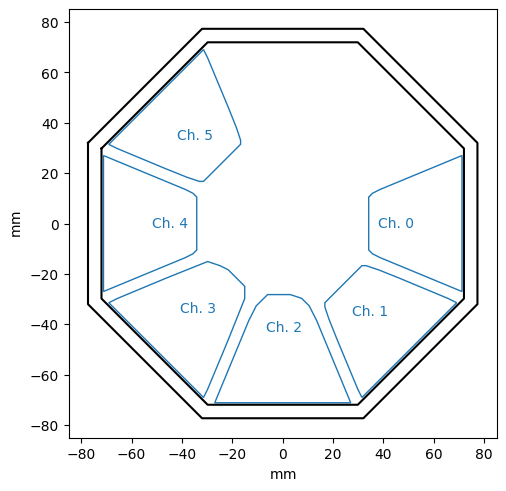
Now, we are ready to plot a footprint diagram of the beam on the primary mirror.

with astropy.visualization.quantity_support():
    fig, ax = plt.subplots(constrained_layout=True)
    instrument_full.schematic_primary(
        ax=ax,
        transformation=transformation,
    )
    ax.set_aspect("equal")